- A series on DR for dummies on medium part 1 2 3
- A small blog post about PCA, AE & TSNE in tensorflow
- Visualizing PCA/TSNE using plots
- Parallex by uber for tsne \ pca visualization
- About tsne / ae / pca
- Does dim-reduction loses information - yes and no, in pca yes only if you use less than the entire matrix
- Performance comparison between dim-reduction implementations, tsne etc.

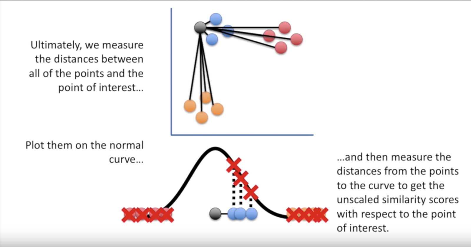
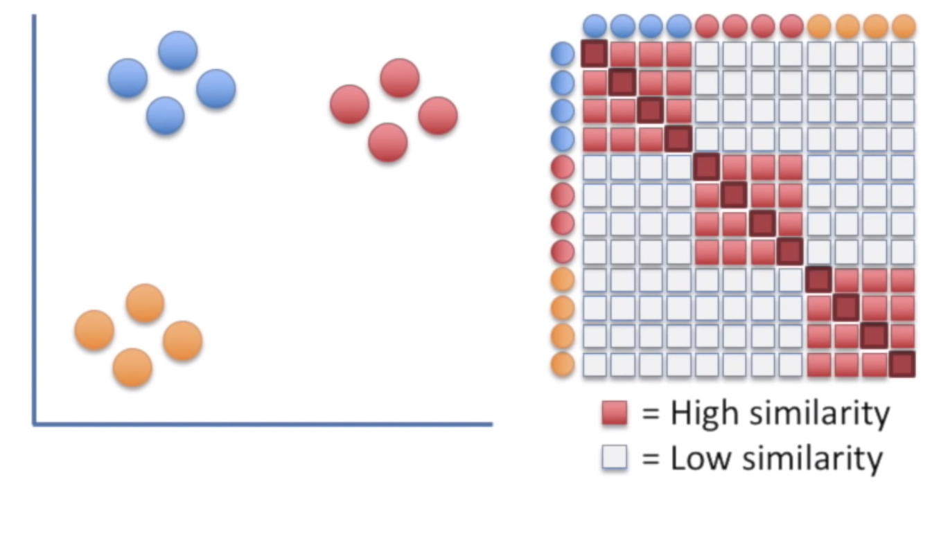
- Stat quest - the jist of it is that we assume a t- distribution on distances and remove those that are farther.normalized for density. T-dist used so that clusters are not clamped in the middle.
Iteratively moving from the left to the right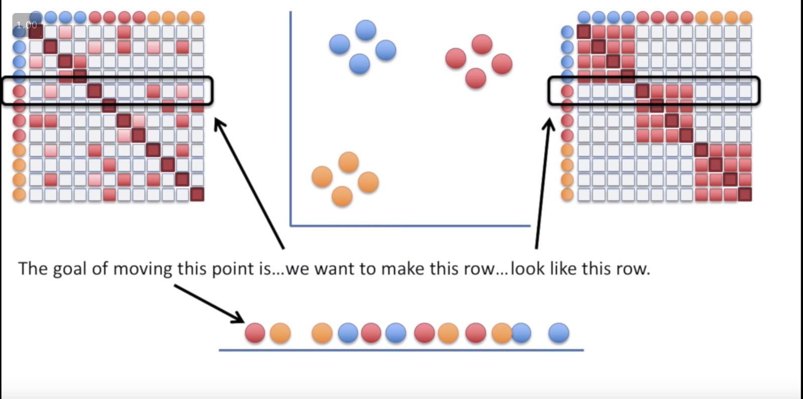
- TSNE algorithm
- Are there cases where PCA more suitable than TSNE
- PCA preserving pairwise distances over tSNE? How why, all here.
- Another advice about using tsne and the possible misinterpetations
- Machine learning mastery:
- Expected value, variance, covariance
- PCA (remove the mean from A, calculate cov(A), calculate eig(cov), A*eigK = PCA)
- EigenDecomposition - what is an eigen vector - simply put its a vector that satisfies A*v = lambda*v, how to use eig() and how to confirm an eigenvector/eigenvalue and reconstruct the original A matrix.
- SVD
- What is missing is how the EigenDecomposition is calculated.
- PCA on large matrices!
- Randomized svd
- Incremental svd
- PCA on Iris
- (did not read) What is PCA?
- (did not read) What is a covariance matrix?
- (did not read) Variance covariance matrix
- Visualization of the first PCA vectors, it is unclear what he is trying to show.
- A very nice introductory tutorial on how to use PCA
- ** An in-depth tutorial on PCA (paper)
- ** yet another tutorial paper on PCA (looks good)
- How to use PCA in Cross validation and for train\test split. (bottom line, do it on the train only.)
- Another tutorial paper - looks decent
- PCA whitening, Stanford tutorial (pca/zca whitening), Stackoverflow (really good) ,
There are two things we are trying to accomplish with whitening:
- Make the features less correlated with one another.
- Give all of the features the same variance.
Whitening has two simple steps:
- Project the dataset onto the eigenvectors. This rotates the dataset so that there is no correlation between the components.
- Normalize the the dataset to have a variance of 1 for all components. This is done by simply dividing each component by the square root of its eigenvalue.
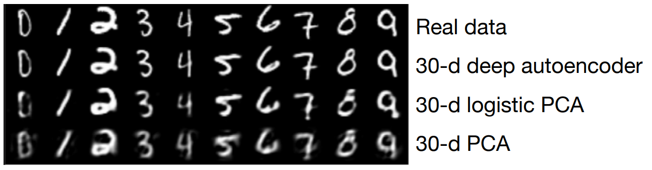
- First they say that Autoencoder is PCA based on their equation, i.e. minimize the reconstruction error formula.
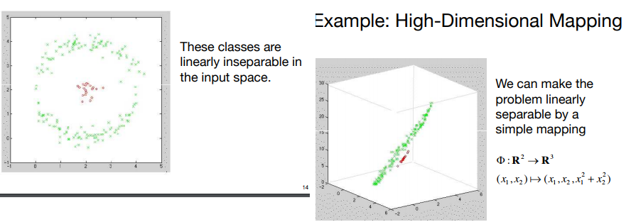
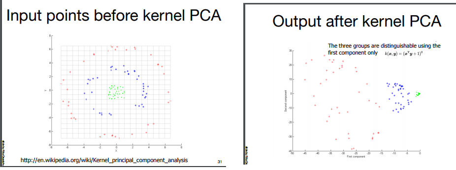
- Then they say that PCA cant separate certain non-linear situations (circle within a circle), therefore they introduce kernel based PCA (using the kernel trick - like svm) which mapps the space to another linearly separable space, and performs PCA on it,
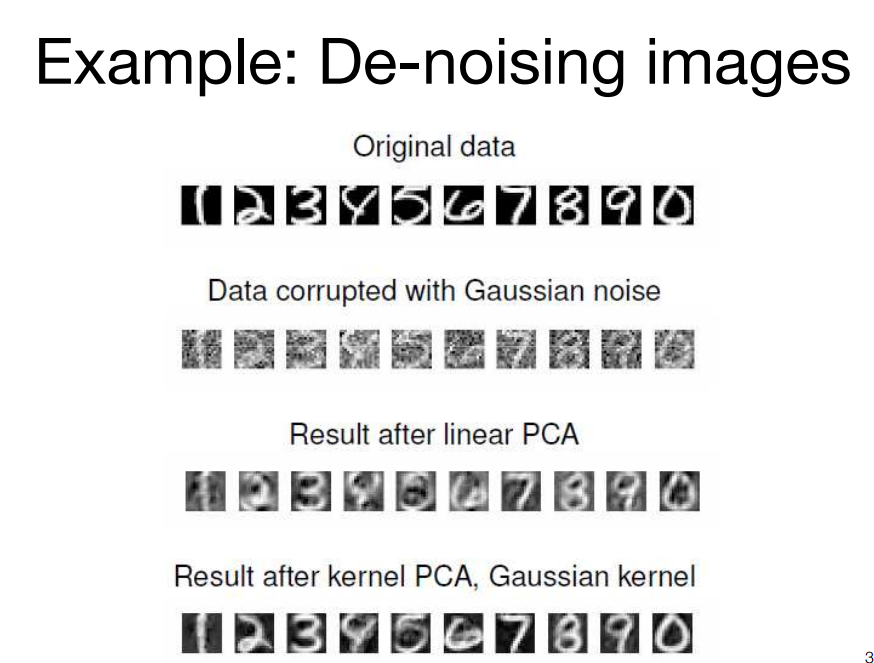
- Finally, showing results how KPCA works well on noisy images, compared to PCA.
A comparison / tutorial with code on pca vs lda - read!
A comprehensive tutorial on LDA - read!
Dim reduction with LDA - nice examples\
(Not to be confused with the other LDA) - Linear Discriminant Analysis (LDA) is most commonly used as dimensionality reduction technique in the pre-processing step for pattern-classification and machine learning applications. The goal is to project a dataset onto a lower-dimensional space with good class-separability in order avoid overfitting (“curse of dimensionality”) and also reduce computational costs.\
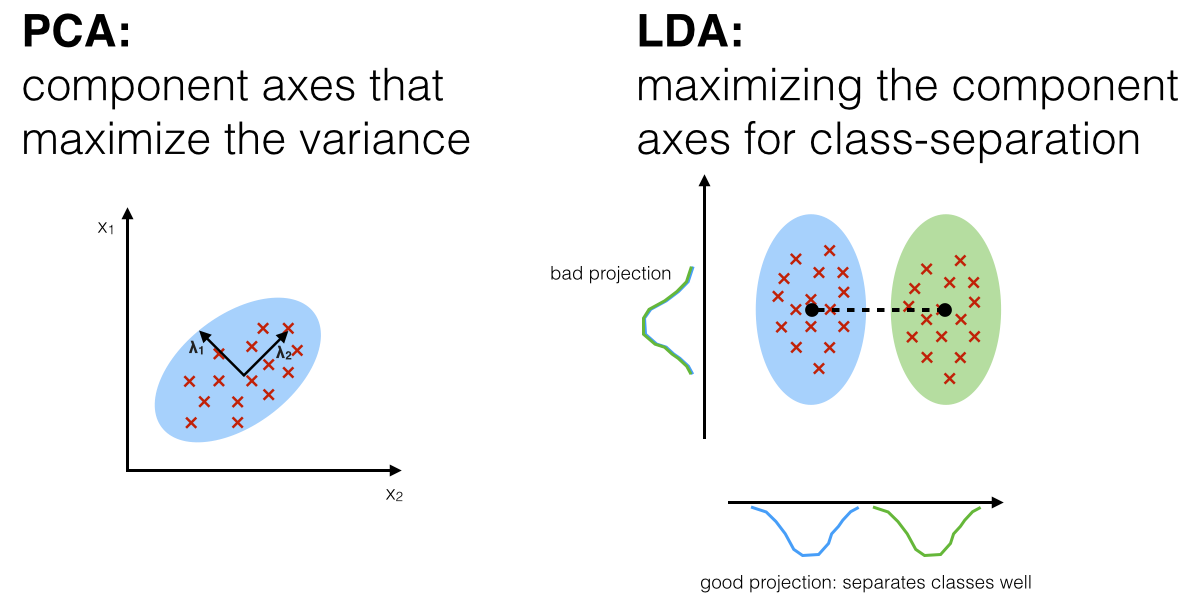
PCA vs LDA:
Both Linear Discriminant Analysis (LDA) and Principal Component Analysis (PCA) are linear transformation techniques used for dimensionality reduction.
- PCA can be described as an “unsupervised” algorithm, since it “ignores” class labels and its goal is to find the directions (the so-called principal components) that maximize the variance in a dataset.
- In contrast to PCA, LDA is “supervised” and computes the directions (“linear discriminants”) that will represent the axes that maximize the separation between multiple classes.
Although it might sound intuitive that LDA is superior to PCA for a multi-class classification task where the class labels are known, this might not always the case.
For example, comparisons between classification accuracies for image recognition after using PCA or LDA show that :
- PCA tends to outperform LDA if the number of samples per class is relatively small (PCA vs. LDA, A.M. Martinez et al., 2001).
- In practice, it is also not uncommon to use both LDA and PCA in combination:
Best Practice: PCA for dimensionality reduction can be followed by an LDA. But before we skip to the results of the respective linear transformations, let us quickly recapitulate the purposes of PCA and LDA: PCA finds the axes with maximum variance for the whole data set where LDA tries to find the axes for best class separability. In practice, often a LDA is done followed by a PCA for dimensionality reduction.
** To fully understand the details please follow the LDA link to the original and very informative article\
*** TODO: need some benchmarking for PCA\LDA\LSA\ETC..
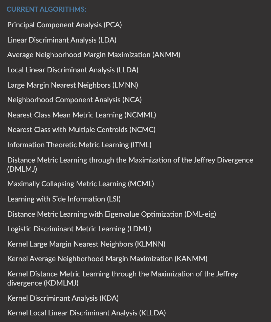
- pyDML package - has KDA - This package provides the classic algorithms of supervised distance metric learning, together with some of the newest proposals.
LSA is quite simple, you just use SVD to perform dimensionality reduction on the tf-idf vectors–that’s really all there is to it! And LSA CLUSTERING\
Here is a very nice tutorial about LSA, with code, explaining what are the three matrices, word clustering, sentence clustering and vector importance. They say that for sentence space we need to remove the first vector as it is correlated with sentence length.\
*how to interpret LSA vectors\
PCA vs LSA: (intuition1, intuition2)
- reduction of the dimensionality
- noise reduction
- incorporating relations between terms into the representation.
- SVD and PCA and "total least-squares" (and several other names) are the same thing. It computes the orthogonal transform that decorrelates the variables and keeps the ones with the largest variance. There are two numerical approaches: one by SVD of the (centered) data matrix, and one by Eigen decomposition of this matrix "squared" (covariance).
- While PCA is global, it finds global variables (with images we get eigen faces, good for reconstruction) that maximizes variance in orthogonal directions, and is not influenced by the TRANSPOSE of the data matrix.
- On the other hand, ICA is local and finds local variables (with images we get eyes ears, mouth, basically edges!, etc), ICA will result differently on TRANSPOSED matrices, unlike PCA, its also “directional” - consider the “cocktail party” problem. On documents, ICA gives topics.
- It helps, similarly to PCA, to help us analyze our data.
Sparse info on ICA with security returns.
- The best tutorial that explains manifold (high to low dim projection/mapping/visuzation) (pca, sammon, isomap, tsne)
- Many manifold methods used to visualize high dimensional data.
- Comparing manifold methods
- Code and in-depth tutorial on TSNE, mapping probabilities to distributions****
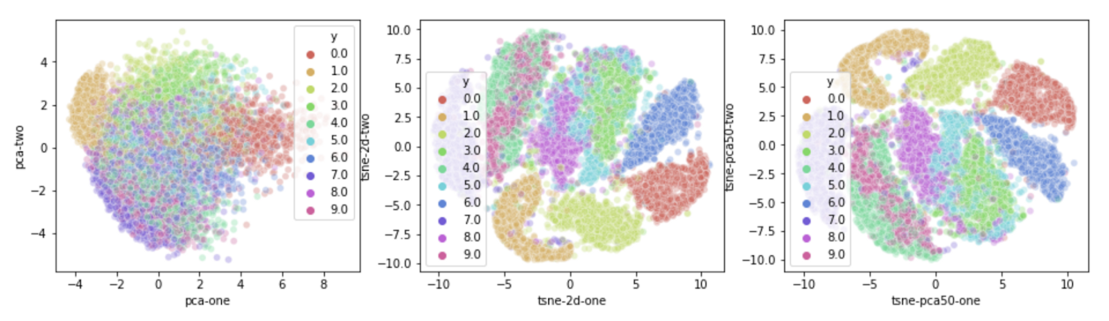
- A great example of using PCA and then TSNE to see clusters that arent visible with PCA only.
- Misreading T-SNE, this is a very important read.
- In contrary to what it says on sklearn’s website, TSNE is not suited ONLY for visualization, you can also use it for data reduction
- “t-Distributed Stochastic Neighbor Embedding (t-SNE) is a (prize-winning) technique for dimensionality reduction that is particularly well suited for the visualization of high-dimensional datasets.”
- Comparing PCA and TSNE, then pushing PCA to TSNE and seeing what happens (as recommended in SKLEARN
- TSNE + AUTOENCODER example